Lab 1.2: Teach It 1s and 2s First, Then Introduce 3 — Watching Weights Reorganize

MNIST internals series. In Lab 1.1 we established what a weight row is: a learned photograph of a class, contrast-carved against its rivals, painted by the update rule $W_c \leftarrow W_c - \eta\,\tfrac1N\sum (\hat p_c - y_c)\,x^\top$ .

Now the experiment that motivated the series: start the model in an impoverished world — only 1s and 2s exist — then let it discover 3. This is continual learning in miniature, and it lets us watch, directly and quantitatively:

1. Phase 1 — what two-class training actually creates (spoiler: the two rows come out near-mirror images, and that’s not an accident),
2. Phase 2 — how the old rows are re-carved when a new class arrives (the “1s/2s accuracy barely moves, but the weights definitely do” effect),
3. Phase 3 — catastrophic forgetting: teach it only 3s afterwards and watch knowledge of 1 and 2 get actively repurposed, not merely fade; then the one-line fix (rehearsal).

Everything is the Lab 1.1 machinery: one softmax layer, plain SGD, float64 NumPy, checkpoints at every phase boundary.

0. Setup

Same model as Lab 1.1, verbatim — the only laboratory instrument here is the dataset’s class composition. First, slice the data down to a two-class universe: all 1s and 2s, relabeled to output indices 0 and 1.

from pathlib import Path
import sys, time
import numpy as np
import matplotlib.pyplot as plt

%matplotlib inline
plt.rcParams["figure.dpi"] = 110

from mnist_lab import (load_mnist, filter_classes, one_hot, show_grid, show_templates,
                       show_confusion, save_fig, save_ckpt, load_ckpt, manifest)

rng = np.random.default_rng(7)
x_train, y_train, x_test, y_test = load_mnist("data")
CKPT = Path("checkpoints/lab02"); FIGS = Path("figures/lab02"); FIGS.mkdir(parents=True, exist_ok=True)

class SoftmaxReg:
    """z = x @ W.T + b ; p = softmax(z) ; cross-entropy loss ; plain SGD. (Verbatim from Lab 1.1.)"""
    def __init__(self, n_in, n_classes, rng, scale=0.01):
        self.W = rng.normal(0, scale, size=(n_classes, n_in))
        self.b = np.zeros(n_classes)
    def logits(self, x):    return x @ self.W.T + self.b
    def probs(self, x):
        z = self.logits(x); z = z - z.max(axis=1, keepdims=True)
        e = np.exp(z); return e / e.sum(axis=1, keepdims=True)
    def loss(self, x, y):
        p = self.probs(x)
        return float(-np.log(p[np.arange(len(y)), y] + 1e-12).mean())
    def grad(self, x, y):
        p = self.probs(x)
        delta = p - one_hot(y, self.W.shape[0])
        return delta.T @ x / len(y), delta.mean(axis=0)
    def step(self, x, y, lr):
        gW, gb = self.grad(x, y)
        self.W -= lr * gW; self.b -= lr * gb
    def predict(self, x):   return self.logits(x).argmax(axis=1)
    def accuracy(self, x, y): return float((self.predict(x) == y).mean())

def per_class_acc(m, x, y, k):
    pred = m.predict(x)
    return [float((pred[y == c] == c).mean()) for c in range(k)]

def cos(u, v): return float(u @ v / (np.linalg.norm(u) * np.linalg.norm(v)))

CLASSES_12 = [1, 2]
xtr12, ytr12, _ = filter_classes(x_train, y_train, CLASSES_12)
xte12, yte12, _ = filter_classes(x_test, y_test, CLASSES_12)
print(f"two-class universe: train {xtr12.shape[0]} {np.bincount(ytr12)}, test {xte12.shape[0]}")

model = SoftmaxReg(784, 2, rng)
BATCH, LR, EPOCHS = 256, 0.5, 3
t0 = time.perf_counter()
for epoch in range(EPOCHS):
    perm = rng.permutation(len(xtr12))
    perm = perm[: len(perm) // BATCH * BATCH]
    for i in perm.reshape(-1, BATCH):
        model.step(xtr12[i], ytr12[i], LR)
acc12 = model.accuracy(xte12, yte12)
print(f"trained {EPOCHS} epochs in {time.perf_counter()-t0:.1f}s | test accuracy on {{1,2}}: {acc12:.2%}")
save_ckpt(CKPT, "phase1_ones_twos", metrics={"test_acc_12": round(acc12, 4)}, W=model.W, b=model.b)

two-class universe: train 12700 [6742 5958], test 2167
trained 3 epochs in 0.1s | test accuracy on {1,2}: 99.22%





PosixPath('checkpoints/lab02/phase1_ones_twos.npz')

1. Two-class weights are mirror images

Theory first: softmax is invariant to adding the same constant to all logits, $p = \mathrm{softmax}(z) = \mathrm{softmax}(z + c\mathbf{1})$ . So the model is free to slide both rows up and down together — only differences of rows drive predictions. With two classes, the entire decision is one scalar: $z_2 - z_1 = (W_2 - W_1)\cdot x + (b_2 - b_1) \gtrless 0$ . The cheapest way to encode “1 vs 2” is therefore a single direction $\pm d$ : row “2” $= +d$ , row “1” $= -d$ .

SGD, converging near the minimum-norm solution, goes exactly there. Let’s measure it.

wA, wB = model.W    # row A = template of digit 1, row B = template of digit 2
print(f"cosine(row_1, row_2)              = {cos(wA, wB):+.4f}")
print(f"||row_1 + row_2|| / ||row_1||     = {np.linalg.norm(wA + wB) / np.linalg.norm(wA):.3f}   (0 = perfectly antisymmetric)")

fig, axes = plt.subplots(1, 3, figsize=(10, 3.1))
for ax, v, ttl in ((axes[0], wA, "template of 1"),
                   (axes[1], wB, "template of 2"),
                   (axes[2], wA + wB, "sum of the two rows")):
    lim = np.abs(v).max()
    ax.imshow(v.reshape(28, 28), cmap="RdBu", vmin=-lim, vmax=lim)
    ax.set_title(ttl, fontsize=9); ax.axis("off")
fig.suptitle("one direction in 784-D space, stored as ±two rows — their sum is nearly nothing")
fig.tight_layout(); save_fig(fig, FIGS / "phase1_mirror.png"); plt.show()

cosine(row_1, row_2)              = -0.9766
||row_1 + row_2|| / ||row_1||     = 0.218   (0 = perfectly antisymmetric)
saved figure -> figures/lab02/phase1_mirror.png

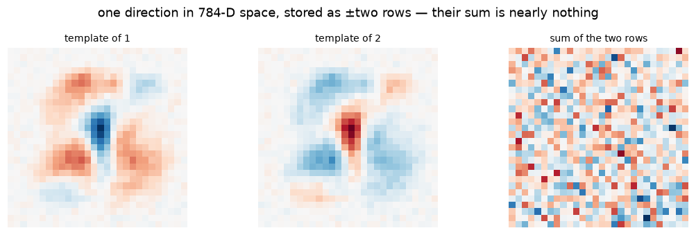
The residual mass in “sum of the two rows” is the shared structure all digits have (the central ink channel) — useless for telling them apart, so it goes un-learned. Weights record contrast, not appearance.

What does this model do with a 3?

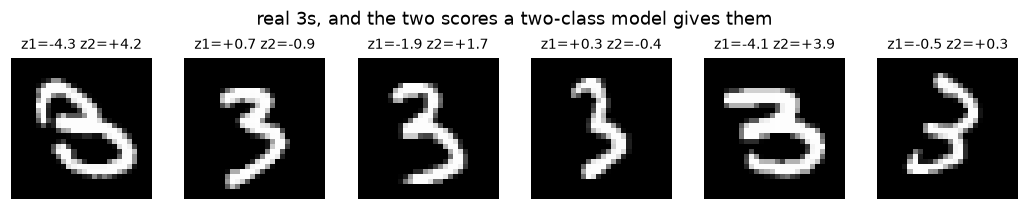
It has no “I don’t know” neuron. A 3 must come out as 1 or 2. Purely from pixel overlap you’d guess most 3s get called “2” — the loops sit in the same places. Let’s check.

x3 = x_test[y_test == 3]
p3 = model.predict(x3)
print("what the {1,2}-model calls every handwritten 3 in the test set:")
print(f"  -> classified as 1: {(p3 == 0).mean():.1%}")
print(f"  -> classified as 2: {(p3 == 1).mean():.1%}")
z3 = model.logits(x3)
print(f"  median logit margin z_2 - z_1 = {np.median(z3[:, 1] - z3[:, 0]):+.2f}")

fig = show_grid(x3[:6], titles=[f"z1={a:+.1f} z2={b:+.1f}" for a, b in z3[:6]], ncols=6,
                suptitle="real 3s, and the two scores a two-class model gives them")
save_fig(fig, FIGS / "threes_in_a_two_class_world.png"); plt.show()

what the {1,2}-model calls every handwritten 3 in the test set:
  -> classified as 1: 23.7%
  -> classified as 2: 76.3%
  median logit margin z_2 - z_1 = +2.40


saved figure -> figures/lab02/threes_in_a_two_class_world.png

2. Introduce the 3

Now add a third output row (random init ~ N(0, 0.01)) and keep training on all of {1, 2, 3} — old rows are NOT frozen, they keep moving. What should we expect?

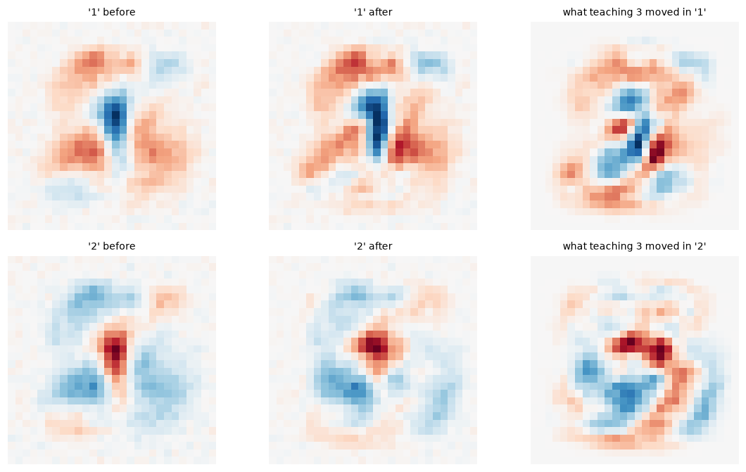
The 2 and the 3 share real estate: both draw a right-side vertical-ish stroke and middle curves. Before 3 arrived, row “2”’s blueprint covered a lot of “3-ish” pixels positively. Once 3s are in the training data, every 3 that scores high on row “2” paints $-\hat p_2\,x$ there (the gradient rule from Lab 1.1). Watch the per-class accuracies, then look at the before/after templates and the change map $\Delta W$ .

CLASSES_123 = [1, 2, 3]
xtr, ytr, _ = filter_classes(x_train, y_train, CLASSES_123)
xte, yte, _ = filter_classes(x_test, y_test, CLASSES_123)

W_before = model.W.copy()

model3 = SoftmaxReg(784, 3, rng)
model3.W = np.vstack([model.W, rng.normal(0, 0.01, (1, 784))])   # keep old rows, append a blank-ish one
model3.b = np.append(model.b, 0.0)

hist = [(0, *per_class_acc(model3, xte, yte, 3))]
step = 0
for epoch in range(1, 4):
    perm = rng.permutation(len(xtr))
    perm = perm[: len(perm) // BATCH * BATCH]
    for i in perm.reshape(-1, BATCH):
        model3.step(xtr[i], ytr[i], LR)
        step += 1
    accs = per_class_acc(model3, xte, yte, 3)
    hist.append((step, *accs))
    save_ckpt(CKPT, f"phase2_epoch{epoch}", step=step,
              metrics={f"acc_{c}": round(a, 4) for c, a in zip(CLASSES_123, accs)},
              W=model3.W, b=model3.b)

print("  step |  acc(1)   acc(2)   acc(3)")
for s, a1, a2, a3 in hist:
    print(f"{s:>6} |  {a1:.4f}   {a2:.4f}   {a3:.4f}")

  step |  acc(1)   acc(2)   acc(3)
     0 |  0.9938   0.9903   0.0297
    73 |  0.9921   0.9641   0.9743
   146 |  0.9930   0.9516   0.9812
   219 |  0.9912   0.9399   0.9861

W_after = model3.W
fig, axes = plt.subplots(2, 3, figsize=(10.5, 6.2))
pairs = [("'1' before", W_before[0]), ("'1' after", W_after[0]), ("what teaching 3 moved in '1'", W_after[0] - W_before[0]),
         ("'2' before", W_before[1]), ("'2' after", W_after[1]), ("what teaching 3 moved in '2'", W_after[1] - W_before[1])]
for ax, (ttl, v) in zip(axes.flat, pairs):
    lim = np.abs(v).max()
    ax.imshow(v.reshape(28, 28), cmap="RdBu", vmin=-lim, vmax=lim)
    ax.set_title(ttl, fontsize=9); ax.axis("off")
fig.tight_layout(); save_fig(fig, FIGS / "phase2_deltas.png"); plt.show()

fig = show_templates(W_after, row_labels=CLASSES_123, suptitle="the full {1, 2, 3} template set")
save_fig(fig, FIGS / "phase2_templates.png"); plt.show()

for c in range(2):
    print(f"template of '{CLASSES_123[c]}': cos(before, after) = {cos(W_before[c], W_after[c]):+.4f}"
          f" | ||delta||/||W|| = {np.linalg.norm(W_after[c] - W_before[c]) / np.linalg.norm(W_before[c]):.3f}")

pred = model3.predict(xte)
cm3 = np.zeros((3, 3), dtype=int)
for t, p in zip(yte, pred):
    cm3[t, p] += 1
fig, ax = plt.subplots(figsize=(4.8, 4.1))
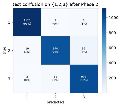
show_confusion(cm3, ["1", "2", "3"], ax=ax, title="test confusion on {1,2,3} after Phase 2")
save_fig(fig, FIGS / "phase2_confusion.png"); plt.show()

saved figure -> figures/lab02/phase2_deltas.png

saved figure -> figures/lab02/phase2_templates.png

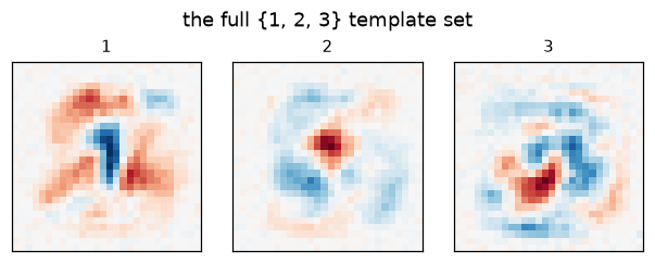
template of '1': cos(before, after) = +0.8990 | ||delta||/||W|| = 0.648
template of '2': cos(before, after) = +0.8431 | ||delta||/||W|| = 0.777
saved figure -> figures/lab02/phase2_confusion.png

Reading Phase 2’s numbers

The accuracies say: teaching 3 was nearly free for 1s (99.4% → 99.1%) but cost the 2s real rent (99.0% → 94.0%), while 3s shot from 2.97% (random new row) to 98.6%. Exactly the digit that shares territory with the newcomer pays.

Meanwhile the templates tell a bigger story: $\|\Delta W\|/\|W\| = 0.65$ for the “1” row and $0.78$ for the “2” row — the matrix was rewritten by more than half its magnitude, and cosine(before, after) fell to 0.90 / 0.84. Same behavior, different weights. The lesson: “the model still gets 99% on 1s and 2s” is a statement about the decision boundary, not about the weights. Net of the cosmetic movement, the Δ-maps show the “2” row ceding middle-right territory to the newborn “3” row.

3. Catastrophic forgetting — and what “forgetting” actually looks like

Now the counterfactual that makes continual learning famous. Roll back to the Phase 1 checkpoint (knows 1s and 2s perfectly, has never seen a 3). Add the third row. Then train on only 3s.

The painting rule predicts something sharper than “the old knowledge fades”: a batch full of 3s applies gradient $-\hat p_c\,x$ to the old rows — they are actively pushed to become “anti-3” detectors. Row 1 and row 2 don’t just decay toward zero; they get repurposed. Measure four things as training proceeds: accuracy on 1s, on 2s, on 3s, and what the old templates look like afterwards.

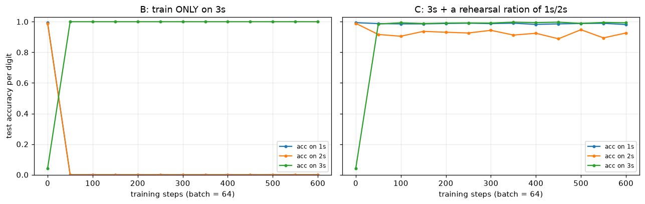
Then rehearsal: same procedure, but each batch is a mixture — mostly 3s plus a small ration of 1s and 2s. One ingredient, and the catastrophe disappears.

base = load_ckpt(CKPT / "phase1_ones_twos.npz")   # roll back: model as of end of Phase 1

def make3():
    m = SoftmaxReg(784, 3, rng)
    m.W = np.vstack([base["W"], np.zeros((1, 784))])   # exact Phase-1 weights + a blank third row
    m.b = np.append(base["b"], 0.0)
    return m

def run_phase(m, xs, ys, steps=600, batch=64, lr=0.2, log_every=50, seed=0):
    r = np.random.default_rng(seed)
    rows = [(0, *per_class_acc(m, xte, yte, 3))]
    for s in range(1, steps + 1):
        i = r.integers(0, len(xs), batch)
        m.step(xs[i], ys[i], lr)
        if s % log_every == 0:
            rows.append((s, *per_class_acc(m, xte, yte, 3)))
    return np.array(rows)

x3tr = x_train[y_train == 3]; y3tr = np.full(len(x3tr), 2)     # only 3s, relabeled index 2

# --- Experiment B: only 3s ---
modelB = make3()
hB = run_phase(modelB, x3tr, y3tr, seed=1)
save_ckpt(CKPT, "phase3B_only3",
          metrics={f"acc_{c}": round(a, 4) for c, a in zip(CLASSES_123, hB[-1, 1:])},
          W=modelB.W, b=modelB.b)

# --- Experiment C: 3s + rehearsal ration of 1s/2s ---
x12_sub, y12_sub = xtr12[::4], ytr12[::4]
xmix = np.concatenate([x3tr, x12_sub]);  ymix = np.concatenate([y3tr, y12_sub])
modelC = make3()
hC = run_phase(modelC, xmix, ymix, seed=1)
save_ckpt(CKPT, "phase3C_rehearsal",
          metrics={f"acc_{c}": round(a, 4) for c, a in zip(CLASSES_123, hC[-1, 1:])},
          W=modelC.W, b=modelC.b)

print("final per-digit test accuracies (start | B: only 3s | C: rehearsal):")
for c, d in enumerate(CLASSES_123):
    print(f"  {d}s: {hB[0, c+1]:.3f} | {hB[-1, c+1]:.3f} | {hC[-1, c+1]:.3f}")

final per-digit test accuracies (start | B: only 3s | C: rehearsal):
  1s: 0.994 | 0.000 | 0.981
  2s: 0.989 | 0.000 | 0.926
  3s: 0.043 | 1.000 | 0.993

fig, axes = plt.subplots(1, 2, figsize=(11.8, 3.8), sharey=True)
for ax, h, ttl in ((axes[0], hB, "B: train ONLY on 3s"),
                   (axes[1], hC, "C: 3s + a rehearsal ration of 1s/2s")):
    for c, d in enumerate(CLASSES_123):
        ax.plot(h[:, 0], h[:, c + 1], "-o", ms=3, lw=1.5, label=f"acc on {d}s")
    ax.set_xlabel("training steps (batch = 64)"); ax.set_title(ttl)
    ax.set_ylim(0, 1.03); ax.grid(alpha=.25); ax.legend(fontsize=8)
axes[0].set_ylabel("test accuracy per digit")
fig.tight_layout(); save_fig(fig, FIGS / "phase3_curves.png"); plt.show()

fig, axes = plt.subplots(1, 5, figsize=(14.5, 2.8))
panels = [(base["W"][0], "'1' after Phase 1"), (modelB.W[0], "'1' after only-3s"),
          (base["W"][1], "'2' after Phase 1"), (modelB.W[1], "'2' after only-3s"),
          (modelB.W[2], "'3' learned in B")]
for ax, (v, ttl) in zip(axes, panels):
    lim = np.abs(v).max()
    ax.imshow(v.reshape(28, 28), cmap="RdBu", vmin=-lim, vmax=lim)
    ax.set_title(ttl, fontsize=9); ax.axis("off")
fig.tight_layout(); save_fig(fig, FIGS / "phase3_templates_B.png"); plt.show()

print("how far the old rows were dragged (cos vs their Phase-1 selves):")
for c, d in ((0, 1), (1, 2)):
    print(f"  row '{d}': {cos(base['W'][c], modelB.W[c]):+.4f}")

saved figure -> figures/lab02/phase3_curves.png

saved figure -> figures/lab02/phase3_templates_B.png

how far the old rows were dragged (cos vs their Phase-1 selves):
  row '1': +0.9748
  row '2': +0.8634

3b. Why did the old knowledge lose? Peek at the numbers

Here is the subtle part that the accuracy curves hide. Compare the old weight rows before and after Experiment B, mechanically — norms, biases, and (already printed above) cosine to their Phase-1 selves:

print("row diagnostics — Phase 1 -> after training on ONLY 3s:")
print("class   ||W||           b")
for c, d in enumerate(CLASSES_123):
    n0 = np.linalg.norm(base["W"][c]) if c < 2 else 0.0
    b0 = float(base["b"][c]) if c < 2 else 0.0
    print(f"  {d}:  {n0:5.2f} -> {np.linalg.norm(modelB.W[c]):5.2f}   {b0:+.2f} -> {modelB.b[c]:+.2f}")

x1 = xte[yte == 0]                       # all real test 1s (class index 0 = digit 1)
z1s = x1 @ modelB.W.T + modelB.b
print(f"\non the {len(x1)} real test 1s:  mean z('1' row) = {z1s[:, 0].mean():+.2f}   z('2' row) = {z1s[:, 1].mean():+.2f}   z('3' row) = {z1s[:, 2].mean():+.2f}")
print(f"the '1' row is still the argmax on {(z1s.argmax(1) == 0).mean():.1%} of them")

row diagnostics — Phase 1 -> after training on ONLY 3s:
class   ||W||           b
  1:   1.79 ->  1.81   +0.14 -> +0.07
  2:   1.81 ->  1.91   -0.14 -> -0.28
  3:   0.00 ->  1.36   +0.00 -> +0.21

on the 1135 real test 1s:  mean z('1' row) = +0.82   z('2' row) = -6.41   z('3' row) = +5.42
the '1' row is still the argmax on 0.0% of them

Neither the directions (cos ≈ 0.97, 0.86) nor the norms (1.8 → 1.8, 1.9) of the old rows were destroyed. Look at the rightmost panel of the figure above instead: the freshly learned “3” template is pure blue — it has no red halo at all. It trained 600 steps on nothing but 3s, so every update painted positive ink, $(1-\hat p_3)\,x$ ; it never once had a rival to suppress.

The old rows, by contrast, carry heavy red halos from their war with each other — so when a real “1” strays a pixel into the old “1” template’s red zone, it pays full price, while the innocent “3” row charges nothing. Result, measured on all 1,135 test 1s: the virgin “3” row scores $z_3 \approx +5.4$ while the actual “1” row ekes out $z_1 \approx +0.8$ (and its mirror, the “2” row, drags $-6.4$ — exactly the antisymmetry from §1 working against itself). Not one test “1” is ever the argmax. The newcomer wins not by knowing more about 3s, but by never having learned to say no.

That is what forgetting is here — not erasure, but out-bidding: the veteran classes’ hard-won red ink turns into a liability the moment an un-criticized class enters the same tournament. Grown-up continual learning has an entire literature on exactly this pathological “new class logit inflation” (e.g. bias correction — Wu et al., BiC, CVPR 2019) and on protecting the red halos (EWC, below).

4. What we actually learned

Softmax rows encode comparisons, not portraits. With two classes the machine literally stores one direction twice with opposite signs — the “sum” panel above is almost blank. The unit of knowledge in $W$ is the boundary between classes, not the class itself.

Adding a class re-carves old weights while barely touching old accuracy. Phase 2: 1s untouched (99.4% → 99.1%), 2s lost ~5 points (99.0% → 94.0%), 3s learned to 98.6% — while the old rows were rewritten by 65–78% of their norm. Knowledge in a neural net is redundant and continuously maintained: many parameter settings classify 1s and 2s equally well, and SGD happily surfs among them when a new demand arrives — silent to any metric that only watches accuracy.

Forgetting here was not erasure — it was out-bidding. After 600 steps of only-3s, accuracy on 1s and 2s was exactly 0%, yet the old rows’ directions survived (cos ≈ 0.97, 0.86) with near-intact norms. The model forgot because the rival-free “3” row — all blue, no suppression halo — outscores the contrast-carved veterans even on their own digits. This is the same pathology large models show when fine-tuning inflates the logits of whatever you trained last: the fix in both worlds is to keep the old knowledge active while the new learns (rehearsal below) or to penalize drift of important weights (EWC).

A trivially small memory of the past prevents it. Rehearsal — a 1-in-4 ration of 1s and 2s mixed into the batch stream — held the old digits at 98.1% / 92.6% while 3s still reached 99.3%. The old rows kept getting their $(1 - \hat p)x$ reinforcement often enough that their red halos survived, so the new class had to grow its own halo too and couldn’t free-ride. Scale this idea up and you get the whole continual-learning toolbox: replay buffers, and its parametric cousin EWC (penalize moving weights that mattered for old tasks).

Curated reading:

• McCloskey & Cohen, Catastrophic Interference in Connectionist Networks (1989) — the original observation.
• French, Catastrophic forgetting in connectionist networks, Trends in Cognitive Sciences (1999).
• Kirkpatrick et al., Overcoming catastrophic forgetting in neural networks (EWC), PNAS 2017 — DeepMind’s weight-importance regularizer.
• On why fine-tuned LLMs forget pretraining skills unless old data is mixed in: same math, larger canvas — the $\hat p - y$ update doesn’t know or care which task an example came from.

Next (Lab 1.3): add a hidden layer. Rows of $W^{(1)}$ stop being digit photographs and become features — edgelets and stroke fragments that no longer correspond to classes — and we will need a new instrument (activation maximization) to see them. That is where the Distill literature begins.

Reproduce

cd labs/ml/mnist-internals
source .venv/bin/activate
jupyter lab     # open 02_teach_1_2_then_3.ipynb

Artifacts: checkpoints/lab02/ (phase1_ones_twos.npz, phase2_epoch{1,2,3}.npz, phase3B_only3.npz, phase3C_rehearsal.npz, + manifest.json), figures/lab02/*.png.

print("checkpoints written this lab:")
for e in manifest(CKPT):
    print(f"  {e['name']:<18} step={str(e['step']):<5} metrics={e['metrics']}")

checkpoints written this lab:
  phase1_ones_twos   step=None  metrics={'test_acc_12': 0.9922}
  phase2_epoch1      step=73    metrics={'acc_1': 0.9921, 'acc_2': 0.9641, 'acc_3': 0.9743}
  phase2_epoch2      step=146   metrics={'acc_1': 0.993, 'acc_2': 0.9516, 'acc_3': 0.9812}
  phase2_epoch3      step=219   metrics={'acc_1': 0.9912, 'acc_2': 0.9399, 'acc_3': 0.9861}
  phase3B_only3      step=None  metrics={'acc_1': 0.0, 'acc_2': 0.0, 'acc_3': 1.0}
  phase3C_rehearsal  step=None  metrics={'acc_1': 0.9815, 'acc_2': 0.9264, 'acc_3': 0.9931}