Lab 2.1: How Word Vectors Learn to Mean — Embeddings From Zero, and What They Secretly Compute
Language-model internals series. In the MNIST series we took apart what weights represent for vision. New series, same ritual — build it from scratch, check gradients numerically, claim nothing without a baseline or a measured number.
The question for this lab, in the plainest possible form:
A word becomes a row of numbers. How can those numbers possibly mean anything?
The answer we will earn, not admire:
- Distributional hypothesis made concrete — we build SGNS (skip-gram with negative sampling) from scratch in NumPy on a microworld corpus whose grammar we control, so every structure claim is checkable against known ground truth (including
king − man + woman ≈ queen— we’ll make it happen from counts alone, and measure how often vector arithmetic actually works). - The reveal — the part most tutorials skip: SGNS is implicitly factorizing a count matrix (the shifted PMI of co-occurrence statistics — Levy & Goldberg, 2014). We will compute that matrix in closed form, scatter what the network learned against what the math says it should learn, and get comparable embeddings without any gradient descent at all, via one SVD of the count matrix.
- Embeddings are mirrors, not minds — a controlled bias experiment: same words, different co-occurrence statistics, watch the geometry move. This is the honest version of all those “word vectors are sexist” headlines.
Prereqs: the embeddings theory note (one-hot → learned table) — we take it from there.
0. A language whose grammar we control
Real corpora (Wikipedia, Shakespeare) are where these ideas get impressive, but they’re where they get unverifiable — you argue from vibes about what the vectors captured. So our corpus is a generated microworld: royalties, commoners, professions, and fruit, with pieces of structure planted deliberately:
- two social tiers — king, queen, prince, princess, duke, duchess, lord, lady vs man, woman, boy, girl, father, mother, son, daughter — each tier having its own exclusive context words (rules the kingdom / throne / crown / court / castle vs field / market / road / garden / river);
- a gender axis carried only by pronoun co-occurrence: male words appear with he/his/him, female with she/her;
- professions that (by default) co-occur with both genders’ pronouns at 50/50 — this will matter in §8;
- an unrelated island: fruit.
If SGNS works at all, the vectors should recover exactly this structure — no more, no less. When it doesn’t, that’s data too.
from pathlib import Path
import sys, time
import numpy as np
import matplotlib.pyplot as plt

%matplotlib inline
plt.rcParams["figure.dpi"] = 110

from lm_lab import (generate_corpus, build_vocab, GENDER_PAIRS, GENDER_OF, ROLE_OF,
                    ENTITY, PROF, FRUIT, save_ckpt, load_ckpt, manifest)

sents = generate_corpus(n_sentences=12000, seed=0)
w2i, vocab, freq = build_vocab(sents)
V = len(vocab)
CKPT = Path("checkpoints/lab21"); FIGS = Path("figures/lab21"); FIGS.mkdir(parents=True, exist_ok=True)

print(f"{len(sents)} sentences, {int(freq.sum())} tokens, vocabulary of {V}")
print()
for s in sents[:6]:
    print("  " + " ".join(s))
print(f"\nmost frequent: {[(vocab[i], int(freq[i])) for i in np.argsort(freq)[::-1][:8]]}")
12000 sentences, 62613 tokens, vocabulary of 85

  the merchant visits the man
  the king sees the duchess today
  the duchess peels a plum
  the man meets the girl
  the queen and the king talk
  the man fishes by the river

most frequent: [('the', 19006), ('her', 1541), ('and', 1332), ('his', 1205), ('duchess', 843), ('talk', 836), ('father', 832), ('duke', 831)]
1. The distributional hypothesis, in table form
Firth (1957): “You shall know a word by the company it keeps.” Take that literally: the “meaning” of a word is its distribution of neighboring words. Below — every word that ever sits within a window of ±2 of king and of queen, counted:
Two things you can already see with your eyes, before any math: their context distributions mirror each other (same throne, same rules, same castle), and the difference is carried by a tiny set of context words (his vs her, he vs she). Everything the embeddings learn later is a compression of facts like these into geometry.
WINDOW = 2
ids = [[w2i[w] for w in s] for s in sents]

# word2vec's subsampling of frequent words (Mikolov 2013, §2.2):
# keep token i with prob min(1, sqrt(t / f_i))  — 'the' at 31% of tokens would otherwise
# dominate every pair (we will see in §3 what that does to training).
# t is a frequency-hyperparameter; the paper's 1e-5..1e-3 is tuned for billion-word
# corpora, we scale it up for our 63k tokens.
T_SUB = 1e-2
f = freq / freq.sum()
keep = np.minimum(1.0, np.sqrt(T_SUB / f))
rng_sub = np.random.default_rng(5)
sub_ids = []
for s in ids:
    kept = [i for i in s if rng_sub.random() < keep[i]]
    if len(kept) >= 3:
        sub_ids.append(kept)
print(f"keep('the')  = {keep[w2i['the']]:.3f}   keep('king') = {keep[w2i['king']]:.3f}")
print(f"tokens: {int(freq.sum()):,} -> {sum(map(len, sub_ids)):,} after subsampling")

pairs = []                                     # (center, context) skip-gram pairs
for s in sub_ids:
    for i, c in enumerate(s):
        for j in range(max(0, i - WINDOW), min(len(s), i + WINDOW + 1)):
            if i != j:
                pairs.append((c, s[j]))
pairs = np.array(pairs)
print(f"{len(pairs):,} (center, context) pairs from window ±{WINDOW}")

def context_counts(word, k=12):
    rows = pairs[pairs[:, 0] == w2i[word]][:, 1]
    u, c = np.unique(rows, return_counts=True)
    order = np.argsort(c)[::-1][:k]
    return [(vocab[u[i]], int(c[i])) for i in order]

print("\ncompany that 'king' keeps:  ", context_counts("king"))
print("\ncompany that 'queen' keeps: ", context_counts("queen"))
keep('the')  = 0.182   keep('king') = 0.896
tokens: 62,613 -> 42,663 after subsampling
102,444 (center, context) pairs from window ±2

company that 'king' keeps:   [('the', 195), ('sees', 86), ('meets', 78), ('and', 76), ('his', 60), ('talk', 58), ('today', 49), ('guards', 41), ('wears', 39), ('carries', 34), ('crown', 32), ('commands', 32)]

company that 'queen' keeps:  [('the', 206), ('sees', 76), ('meets', 74), ('and', 69), ('her', 66), ('today', 53), ('wears', 48), ('talk', 46), ('on', 45), ('sits', 45), ('guards', 40), ('crown', 40)]
2. The count matrix the neural net will secretly factorize
Raw counts are dominated by the (31% of all tokens — it keeps everyone’s company, which is uninformative). The standard fix: pointwise mutual information,
“How much more often do
$w$
and
$c$
co-occur than if they were independent?” — ~0 for the (it co-occurs at the base rate), strongly positive for king/throne. This 85×85 matrix is the complete distributional summary of the corpus. Compute it in closed form and keep it: it is the answer key for what SGNS is about to learn (Levy & Goldberg, 2014 — §5).
C = np.zeros((V, V))
np.add.at(C, (pairs[:, 0], pairs[:, 1]), 1.0)

cw = C.sum(axis=1)                      # how often each word appears as center
cc = C.sum(axis=0)                      # ...and as context
N = C.sum()
with np.errstate(divide="ignore"):
    PMI = np.log(C * N / (cw[:, None] * cc[None, :]))
PMI[C == 0] = -np.inf                    # never seen together -> undefined, handled per-experiment

def top_pmi(word, k=10):
    row = PMI[w2i[word]]
    ok = np.isfinite(row)
    order = np.argsort(np.where(ok, row, -np.inf))[::-1][:k]
    return [(vocab[i], round(float(row[i]), 2)) for i in order]

print("PMI('king', ·):   ", top_pmi("king"))
print("PMI('queen', ·):  ", top_pmi("queen"))
print("PMI('apple', ·):  ", top_pmi("apple"))
row_the = PMI[w2i["the"]]
print("PMI('the', ·):    every finite context sits near 0 — max |PMI| =",
      round(float(np.abs(row_the[np.isfinite(row_the)]).max()), 3))
PMI('king', ·):    [('meets', 1.33), ('guards', 1.33), ('castle', 1.25), ('wears', 1.17), ('crown', 1.15), ('commands', 1.12), ('court', 1.1), ('talk', 1.09), ('rules', 1.09), ('kingdom', 1.04)]
PMI('queen', ·):   [('she', 1.38), ('crown', 1.36), ('wears', 1.36), ('rules', 1.31), ('guards', 1.28), ('meets', 1.26), ('kingdom', 1.25), ('castle', 1.2), ('sits', 1.03), ('on', 1.03)]
PMI('apple', ·):   [('eats', 2.3), ('grows', 2.24), ('a', 2.22), ('is', 2.17), ('peels', 2.17), ('sweet', 1.96), ('in', 1.74), ('orchard', 0.15), ('the', -0.4), ('daughter', -0.45)]
PMI('the', ·):    every finite context sits near 0 — max |PMI| = 4.428
3. SGNS from scratch
The machinery (Mikolov et al., 2013, skip-gram + negative sampling). Two embedding tables — target vectors $E \in \mathbb{R}^{V \times d}$ and context vectors $U \in \mathbb{R}^{V \times d}$ . For each observed pair $(w, c)$ : score $\sigma(E_w \cdot U_c)$ should be high; for $k$ negative pairs $(w, c_j)$ sampled from the unigram distribution (to the 3/4 power, as in the paper), the score should be low:
$$\mathcal{L} = -\sum_{(w,c)} \Big[ \log \sigma(E_w \cdot U_c) \;+\; \sum_{j=1}^{k} \log \sigma(-E_w \cdot U_{c_j}) \Big]$$An honest admission, because it teaches the range of the hyperparameters. The first version of this lab used one 8192-pair synchronous batch and no subsampling. Training diverged to $\|E\| \sim 10^{25}$ within the first epoch — visible salt-and-pepper NaN by epoch 4. The mechanism, in numbers:
theis 31% of the corpus, so it is center or context in the majority of an 8192-pair batch; each of those ~2,000 pairs pushes its row in the same stale direction simultaneously — an effective per-batch step oflr × 2000. Geometric blow-up. The reference implementation avoids this with per-pair (online) updates, and the paper has subsampling precisely to stop the ultra-frequent token from owning the gradient stream. Below: small batches (256, sum-of-gradients — close to online), annealed lr, subsampled stream. Wall time: ~3 seconds for 10 epochs.
Each term is just logistic regression on a dot product, so the gradients are immediate:
$$\frac{\partial}{\partial E_w} = (\sigma(s) - 1)\,U_c + \sum_j \sigma(s_j)\,U_{c_j}, \qquad s = E_w U_c^\top$$…and symmetric for the $U$ side. Ritual first: finite-difference check on a single pair (same ceremony as the MNIST labs), then a vectorized batch trainer that must produce identical gradients to the slow pairwise version — an exact-consistency assert, stronger than the numeric check.
def sigmoid(x):    return 1.0 / (1.0 + np.exp(-np.clip(x, -30, 30)))   # clip: gradients saturate long before ±30
def logsigmoid(x): return -np.logaddexp(0.0, -x)

def loss_pair(E, U, w, c, negs):
    return float(-(logsigmoid(E[w] @ U[c]) + sum(logsigmoid(-E[w] @ U[j]) for j in negs)))

def grad_pair(E, U, w, c, negs):
    """Analytic gradients for ONE pair. Returns (gE_w, gU_c, {neg_id: gU_neg})."""
    s_pos = sigmoid(E[w] @ U[c]) - 1.0                 # d log sigmoid / d s
    gE = s_pos * U[c]
    gC = s_pos * E[w]
    gN = {}
    for j in negs:
        s = sigmoid(E[w] @ U[j])                        # d log sigmoid(-s) / d s
        gE += s * U[j]
        gN[j] = gN.get(j, 0.0) + s * E[w]
    return gE, gC, gN

# --- finite-difference ritual ---
r = np.random.default_rng(0)
E0, U0 = r.normal(0, .1, (V, 6)), r.normal(0, .1, (V, 6))
w, c, negs = w2i["king"], w2i["throne"], [w2i["banana"], w2i["her"], w2i["road"]]
gE, gC, gN = grad_pair(E0, U0, w, c, negs)
eps, errs = 1e-6, []
for flat in range(6):
    for M, Mgrad, row in ((E0, gE, w), (U0, gC, c), (U0, gN[w2i["her"]], w2i["her"])):
        orig = M[row, flat]
        M[row, flat] = orig + eps; lp = loss_pair(E0, U0, w, c, negs)
        M[row, flat] = orig - eps; lm = loss_pair(E0, U0, w, c, negs)
        M[row, flat] = orig
        errs.append(abs(Mgrad[flat] - (lp - lm) / (2 * eps)))
print(f"finite-difference check on 18 scalar entries: max abs error = {max(errs):.2e}")
finite-difference check on 18 scalar entries: max abs error = 4.20e-10
# Strict version of the consistency claim: one pair through the vectorized math == grad_pair
B = 1
rngc = np.random.default_rng(11)
Ec = rngc.normal(0, .1, (V, 4)); Uc = rngc.normal(0, .1, (V, 4))
w_, c_, n_ = 3, 17, [5, 42]
gE_slow, gC_slow, gN_slow = grad_pair(Ec, Uc, w_, c_, n_)

Ew, Ucc = Ec[[w_]], Uc[[c_]]
Un = Uc[n_][None, :, :]
g_pos = sigmoid((Ew * Ucc).sum(1)) - 1
g_neg = sigmoid((Ew[:, None, :] * Un).sum(2))
gEw = (g_pos[:, None] * Ucc + (g_neg[:, :, None] * Un).sum(1))[0]
gUc2 = (g_pos[:, None] * Ew)[0]
print(f"|gE_vec - gE_pair|   = {np.abs(gEw - gE_slow).max():.2e}")
print(f"|gUc_vec - gUc_pair| = {np.abs(gUc2 - gC_slow).max():.2e}")
for j, g in gN_slow.items():
    print(f"|gUn[{j}]_vec - gUn_pair| = {np.abs(g_neg[0, list(n_).index(j)] * Ec[w_] - g).max():.2e}")
|gE_vec - gE_pair|   = 6.94e-18
|gUc_vec - gUc_pair| = 0.00e+00
|gUn[5]_vec - gUn_pair| = 0.00e+00
|gUn[42]_vec - gUn_pair| = 0.00e+00
def train_sgns(pairs, freq, d, k=5, epochs=10, lr=0.05, batch=256, seed=1, verbose=True):
    rng = np.random.default_rng(seed)
    E = rng.normal(0, 0.02, (V, d))
    U = np.zeros((V, d))                              # word2vec convention: context table starts at 0
    p_neg = freq ** 0.75                              # negatives from FULL unigram^0.75, as in the paper
    p_neg /= p_neg.sum()
    probe = pairs[rng.integers(0, len(pairs), 256)]   # fixed probe set for the loss curve
    probe_neg = rng.choice(V, (256, k), p=p_neg)

    t0 = time.perf_counter()
    for ep in range(1, epochs + 1):
        perm = rng.permutation(len(pairs))
        neg = rng.choice(V, (len(pairs), k), p=p_neg)
        lr_t = lr * (1 - (ep - 1) / epochs)           # anneal to 0, like the reference implementation
        for b in range(0, len(pairs), batch):
            idx = perm[b:b + batch]
            w, c = pairs[idx, 0], pairs[idx, 1]
            n = neg[idx]
            n = np.where(n == c[:, None], (n + 1) % V, n)

            Ew, Uc = E[w], U[c]                        # gather BEFORE any update (consistent gradients)
            Un = U[n.reshape(-1)].reshape(len(idx), k, d)
            g_pos = sigmoid((Ew * Uc).sum(1)) - 1.0
            g_neg = sigmoid((Ew[:, None, :] * Un).sum(2))
            gEw = g_pos[:, None] * Uc + (g_neg[:, :, None] * Un).sum(1)
            gUc = g_pos[:, None] * Ew
            gUn = g_neg[:, :, None] * Ew[:, None, :]
            np.add.at(E, w, -lr_t * gEw)
            np.add.at(U, c, -lr_t * gUc)
            np.add.at(U, n.ravel(), -lr_t * gUn.reshape(-1, d))
        if verbose:
            tot = float(np.mean([loss_pair(E, U, int(w0), int(c0), n0) for w0, c0, n0 in zip(probe[:, 0], probe[:, 1], probe_neg)]))
            print(f"epoch {ep:>2}: probe loss {tot:.4f}")
    if verbose:
        print(f"trained d={d} for {epochs} epochs on {len(pairs):,} pairs in {time.perf_counter() - t0:.0f}s")
    return E, U

D = 16
E, U = train_sgns(pairs, freq, D, epochs=10, lr=0.05, seed=1)
epoch  1: probe loss 1.7383


epoch  2: probe loss 1.7077


epoch  3: probe loss 1.7400


epoch  4: probe loss 1.6109


epoch  5: probe loss 1.6520


epoch  6: probe loss 1.5941


epoch  7: probe loss 1.5983


epoch  8: probe loss 1.5982


epoch  9: probe loss 1.5518


epoch 10: probe loss 1.5469
trained d=16 for 10 epochs on 102,444 pairs in 1s
4. Geometry from nowhere
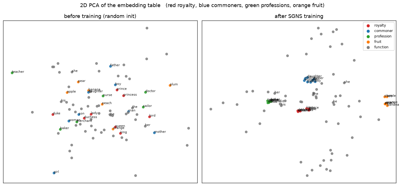
Watch the embedding space before and after training, projected onto its first two principal components (plain SVD of the centered $E$ — 4 lines, no sklearn). Colors are the roles we planted by hand: royalty, commoners, professions, fruit. Then the blast-radius table: nearest neighbors by cosine before and after.
def normed(M):
    n = np.linalg.norm(M, axis=1, keepdims=True)
    return M / np.maximum(n, 1e-12)

def neighbors(E, word, k=8, exclude=()):
    E0 = normed(E)
    sims = E0 @ E0[w2i[word]]
    out = []
    for i in np.argsort(sims)[::-1]:
        if vocab[i] != word and vocab[i] not in exclude:
            out.append((vocab[i], round(float(sims[i]), 3)))
        if len(out) == k:
            return out

print("neighbors of king  (after):", neighbors(E, "king"))
print("neighbors of queen (after):", neighbors(E, "queen"))
print("neighbors of apple (after):", neighbors(E, "apple"))
print("neighbors of the   (after):", neighbors(E, "the"))
neighbors of king  (after): [('lord', 0.995), ('duke', 0.994), ('prince', 0.994), ('duchess', 0.814), ('lady', 0.795), ('queen', 0.793), ('princess', 0.792), ('boy', 0.486)]
neighbors of queen (after): [('princess', 0.996), ('lady', 0.994), ('duchess', 0.992), ('king', 0.793), ('lord', 0.79), ('duke', 0.775), ('prince', 0.759), ('him', 0.552)]
neighbors of apple (after): [('plum', 0.997), ('pear', 0.994), ('orange', 0.992), ('peach', 0.989), ('banana', 0.988), ('orchard', 0.581), ('ripe', 0.57), ('works', 0.528)]
neighbors of the   (after): [('today', 0.392), ('at', 0.35), ('coat', 0.336), ('father', 0.301), ('wage', 0.294), ('girl', 0.281), ('woman', 0.272), ('a', 0.271)]
ROLES = {"royalty": "tab:red", "commoner": "tab:blue", "profession": "tab:green",
         "fruit": "tab:orange", "function": "grey"}
def role_of(w): return ROLE_OF.get(w, "function")

def pca2(M):
    X = M - M.mean(0)
    _, S, Vt = np.linalg.svd(X, full_matrices=False)
    return X @ Vt[:2].T, S

fig, axes = plt.subplots(1, 2, figsize=(13, 6))
Ernd = np.random.default_rng(1).normal(0, 0.02, (V, D))
for ax, M, ttl in ((axes[0], Ernd, "before training (random init)"), (axes[1], E, "after SGNS training")):
    P, _ = pca2(M)
    for i, w in enumerate(vocab):
        ax.scatter(P[i, 0], P[i, 1], color=ROLES[role_of(w)], s=26, alpha=.85)
        if w in ENTITY or w in ("the", "he", "she", "his", "her"):
            ax.annotate(w, (P[i, 0], P[i, 1]), fontsize=7, alpha=.9)
    ax.set_title(ttl); ax.set_xticks([]); ax.set_yticks([])
for role, color in ROLES.items():
    axes[1].scatter([], [], color=color, label=role)
axes[1].legend(fontsize=8, loc="best")
fig.suptitle("2D PCA of the embedding table   (red royalty, blue commoners, green professions, orange fruit)")
fig.tight_layout(); save_fig = lambda f, p: (f.savefig(p, dpi=140, bbox_inches="tight"), print("saved ->", p))
save_fig(fig, FIGS / "pca_before_after.png"); plt.show()
saved -> figures/lab21/pca_before_after.png
5. The reveal: SGNS is a count-matrix factorization in a trench coat
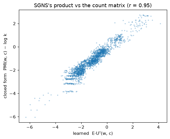
Levy & Goldberg (2014, Neural Word Embedding as Implicit Matrix Factorization) proved that SGNS’s global optimum, when $d$ is large enough, satisfies
$$E \cdot U^\top \;=\; \mathrm{PMI}(w, c) - \log k$$i.e. the product of the two learned tables is the PMI matrix from §2, shifted by $\log k$ ( $k$ = negatives per pair). Two tests we can run ourselves:
Test A — the learned product vs the closed form. Scatter $M = E U^\top$ against $\mathrm{PMI} - \log k$ on the observed pairs and measure the correlation. Our $d=16$ (with $V=85$ and an effective rank well above 16) means we should get a good but imperfect match — and that’s interesting, not disappointing.
Test B — skip the neural net entirely. Factorize the shifted matrix directly: take the positive part $\mathrm{SPPMI} = \max(\mathrm{PMI} - \log k, 0)$ , one SVD, keep the top 16 components: $E_{\mathrm{SVD}} = U\Sigma^{1/2}$ . No gradients, no sampling, no epochs.
A prediction and its honest caveat: where co-occurrence mass is dense (our profession and fruit islands), the two should agree well. Where the matrix is sparse — 2,087 observed pairs fill only 29% of it — the SVD has to assign the unobserved zeros the same weight as observed ones, while SGD only ever saw observed positives and sampled negatives: effectively a weighted factorization that ignores unobserved cells. (Weighting the count matrix is exactly the insight GloVe was built on.) So expect agreement on islands, disagreement on highly-mixed words — and that disagreement is instructive, not a defect.
k_neg = 5
shifted = PMI - np.log(k_neg)
obs = C > 0

M = E @ U.T
x, y = M[obs], shifted[obs]
r = float(np.corrcoef(x, y)[0, 1])
print(f"Test A: corr(E·Uᵀ,  PMI − log k) over {obs.sum()} observed pairs:  r = {r:.3f}")

fig, ax = plt.subplots(figsize=(5.5, 4.5))
sel = np.random.default_rng(0).choice(int(obs.sum()), min(3000, int(obs.sum())), replace=False)
ax.scatter(x[sel], y[sel], s=3, alpha=.25)
ax.set_xlabel("learned  E·Uᵀ(w, c)"); ax.set_ylabel("closed form  PMI(w, c) − log k")
ax.set_title(f"SGNS's product vs the count matrix (r = {r:.2f})")
fig.tight_layout()
fig.savefig(FIGS / "sgns_vs_pmi.png", dpi=140, bbox_inches="tight"); plt.show()

# --- Test B: closed-form embeddings from one SVD of the shifted-PMI matrix ---
SPPMI = np.maximum(np.nan_to_num(shifted, neginf=-1e9), 0)
Usvd, S, _ = np.linalg.svd(SPPMI)
E_svd = Usvd[:, :D] * np.sqrt(S[:D])

print("\nTest B — nearest neighbors, SVD-of-counts vs trained SGNS:")
for w_ in ("king", "queen", "doctor", "apple"):
    print(f"  {w_:>7} SVD : {[w for w, _ in neighbors(E_svd, w_, 6)]}")
    print(f"  {w_:>7} SGNS: {[w for w, _ in neighbors(E, w_, 6)]}")
S_E, S_S = normed(E) @ normed(E).T, normed(E_svd) @ normed(E_svd).T
cos_models = float(np.corrcoef(S_E[obs], S_S[obs])[0, 1])
print(f"\nneighbor-structure agreement (cos-sim of words, over observed pairs): r = {cos_models:.3f}")
save_ckpt(CKPT, "sgns_main", metrics={"dim": D, "pearson_vs_pmi": round(r, 3)},
          E=E, U=U, vocab=np.array(vocab), PMI=PMI, C=C)
Test A: corr(E·Uᵀ, PMI − log k) over 2087 observed pairs: r = 0.952
Test B — nearest neighbors, SVD-of-counts vs trained SGNS:
     king SVD : ['sits', 'throne', 'on', 'greets', 'road', 'walks']
     king SGNS: ['lord', 'duke', 'prince', 'duchess', 'lady', 'queen']
    queen SVD : ['road', 'walks', 'king', 'meets', 'duchess', 'daughter']
    queen SGNS: ['princess', 'lady', 'duchess', 'king', 'lord', 'duke']
   doctor SVD : ['merchant', 'nurse', 'teacher', 'baker', 'sailor', 'bag']
   doctor SGNS: ['teacher', 'nurse', 'merchant', 'sailor', 'baker', 'kingdom']
    apple SVD : ['banana', 'pear', 'plum', 'orange', 'peach', 'ripe']
    apple SGNS: ['plum', 'pear', 'orange', 'peach', 'banana', 'orchard']

neighbor-structure agreement (cos-sim of words, over observed pairs): r = 0.325


PosixPath('checkpoints/lab21/sgns_main.npz')
6. Do the linear analogies actually work? (Measure, don’t demo)
The famous party trick is $E_{king} - E_{man} + E_{woman} \stackrel{?}{\approx} E_{queen}$ . The usual blog post shows one flattering example. We have ground truth, so instead we can measure the thing and the reason it works, separately:
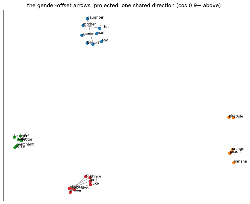
Why it should work: the trick needs “gender” to be one shared direction — the offset vector female − male pointing the same way for every pair. Measure that first: align the eight offset vectors against woman − man.
Why it might still fail at ranking: our microworld has distributional twins — king/prince/duke/lord share identical context distributions by construction, so their vectors are nearly identical (cos ≈ 1.0). When the answer cluster is that tight, the last few percent of per-vector noise decides argmax — the relation can be perfectly parallel while the ranking is a coin flip among near-ties. The famous demos quietly benefit from the forgiving fact that “queen” is the obvious top-1 in a Wikipedia-scale world; on our 60k tokens you’ll see the seam.
Grading is therefore three-tier per quad: exact word, right gender class, right tier. And for the flagship query, we print where queen actually ranks, and by how much it misses.
def analogy(E, a, b, c, k=8):
    E0 = normed(E)
    vec = E0[w2i[b]] - E0[w2i[a]] + E0[w2i[c]]
    vec = vec / np.linalg.norm(vec)
    sims = E0 @ vec
    out = []
    for i in np.argsort(sims)[::-1]:
        if vocab[i] not in (a, b, c):
            out.append((vocab[i], round(float(sims[i]), 3)))
        if len(out) == k:
            return out

# --- why it should work: gender offsets are one shared direction ---
E0 = normed(E)
ref = E0[w2i["woman"]] - E0[w2i["man"]]
print("alignment of each pair's gender offset with (woman - man):")
for m, f_ in GENDER_PAIRS:
    o = E0[w2i[f_]] - E0[w2i[m]]
    print(f"  {m:>8} -> {f_:<9} cos = {o @ ref / np.linalg.norm(o) / np.linalg.norm(ref):+.3f}")

# --- how it does at ranking, graded honestly ---
QUADS = [(m, "man", "woman", f) for m, f in GENDER_PAIRS] \
      + [(f, "woman", "man", m) for m, f in GENDER_PAIRS]
exact = gender = 0
print(f"\n{'quad':<28} {'answer':>9} {'wanted':>9}  exact/gender-ok")
for a, b, c, want in QUADS:
    top = analogy(E, a, b, c)[0][0]
    ex = top == want
    gn = GENDER_OF.get(top) == GENDER_OF[want]
    exact += ex; gender += gn
    print(f"{a + ' - ' + b + ' + ' + c:<28} {top:>9} {want:>9}  {'Y' if ex else 'n'}   {'Y' if gn else 'n'}")
print(f"\nexact answer: {exact}/{len(QUADS)}   right gender: {gender}/{len(QUADS)}")

# the flagship miss, dissected:
res = analogy(E, "king", "man", "woman", k=12)
names = [w for w, _ in res]
qr = names.index("queen") + 1 if "queen" in names else ">12"
print(f"\nking - man + woman: top5 = {names[:5]},  ... queen ranks #{qr}"
      + (f" at cos {res[qr - 1][1]} vs top {res[0][1]}" if qr != '>12' else ""))
alignment of each pair's gender offset with (woman - man):
      king -> queen     cos = +0.987
    prince -> princess  cos = +0.984
      duke -> duchess   cos = +0.981
      lord -> lady      cos = +0.965
       man -> woman     cos = +1.000
       boy -> girl      cos = +0.948
    father -> mother    cos = +0.977
       son -> daughter  cos = +0.945

quad                            answer    wanted  exact/gender-ok
king - man + woman            daughter     queen  n   Y
prince - man + woman          daughter  princess  n   Y
duke - man + woman            daughter   duchess  n   Y
lord - man + woman            daughter      lady  n   Y
man - man + woman               mother     woman  n   Y
boy - man + woman             daughter      girl  n   Y
father - man + woman            mother    mother  Y   Y
son - man + woman             daughter  daughter  Y   Y
queen - woman + man             father      king  n   Y
princess - woman + man          father    prince  n   Y
duchess - woman + man           father      duke  n   Y
lady - woman + man              father      lord  n   Y
woman - woman + man             father       man  n   Y
girl - woman + man                 son       boy  n   Y
mother - woman + man               son    father  n   Y
daughter - woman + man             son       son  Y   Y

exact answer: 3/16   right gender: 16/16

king - man + woman: top5 = ['daughter', 'mother', 'girl', 'father', 'son'],  ... queen ranks #>12
P, _ = pca2(E)
fig, ax = plt.subplots(figsize=(8, 6.5))
for i, w in enumerate(vocab):
    if w in ENTITY:
        ax.scatter(P[i, 0], P[i, 1], color=ROLES[role_of(w)], s=40)
        ax.annotate(w, (P[i, 0], P[i, 1]), fontsize=8)
for m, f_ in GENDER_PAIRS:
    i, j = w2i[m], w2i[f_]
    ax.annotate("", xy=P[j], xytext=P[i],
                arrowprops=dict(arrowstyle="->", color="grey", lw=1.1, alpha=.8))
ax.set_title("the gender-offset arrows, projected: one shared direction (cos 0.9+ above)")
ax.set_xticks([]); ax.set_yticks([])
fig.tight_layout(); fig.savefig(FIGS / "analogy_arrows.png", dpi=140, bbox_inches="tight"); plt.show()
7. How much dimension does “meaning” need?
Repeat training at $d \in \{2, 4, 8, 16, 32, 64\}$ (6 epochs each — enough to compare) and grade three things per dimension: exact-answer analogy accuracy, gender-direction accuracy (the §6 metric that survived contact with reality), and correlation of $EU^\top$ with the shifted-PMI matrix (the §5 yardstick).
The expectation to check: very small $d$ shouldn’t be able to hold BOTH the tier structure and the gender direction… but remember where the noise floor really is — random chance on these quads is around 1-in-20, and the PMI-correlation should keep rising with $d$ until it runs out of rank. Somewhere in this table the microworld becomes honest about how many directions its “meaning” actually uses.
rows = []
for d in (2, 4, 8, 16, 32, 64):
    Ed, Ud = train_sgns(pairs, freq, d, epochs=6, lr=0.05, seed=1, verbose=False)
    topx = [analogy(Ed, a, b, c, k=1)[0][0] for a, b, c, _ in QUADS]
    acc_exact = np.mean([t == want for t, (_, _, _, want) in zip(topx, QUADS)])
    acc_gender = np.mean([GENDER_OF.get(t) == GENDER_OF[want] for t, (_, _, _, want) in zip(topx, QUADS)])
    rr = float(np.corrcoef((Ed @ Ud.T)[obs], shifted[obs])[0, 1])
    rows.append((d, acc_exact, acc_gender, rr))
    print(f"d={d:>2} | exact {acc_exact:0.2f} | gender-dir {acc_gender:0.2f} | corr(E·Uᵀ, PMI−log k) = {rr:.3f}")
save_ckpt(CKPT, "dim_sweep",
          metrics={str(r[0]): {"analogy_exact": round(float(r[1]), 2), "gender_acc": round(float(r[2]), 2),
                               "pearson": round(r[3], 3)} for r in rows})
d= 2 | exact 0.06 | gender-dir 0.12 | corr(E·Uᵀ, PMI−log k) = 0.618


d= 4 | exact 0.00 | gender-dir 0.12 | corr(E·Uᵀ, PMI−log k) = 0.775


d= 8 | exact 0.12 | gender-dir 0.56 | corr(E·Uᵀ, PMI−log k) = 0.911


d=16 | exact 0.12 | gender-dir 1.00 | corr(E·Uᵀ, PMI−log k) = 0.940


d=32 | exact 0.12 | gender-dir 1.00 | corr(E·Uᵀ, PMI−log k) = 0.948


d=64 | exact 0.12 | gender-dir 1.00 | corr(E·Uᵀ, PMI−log k) = 0.956


PosixPath('checkpoints/lab21/dim_sweep.npz')
8. Embeddings are mirrors, not minds
Last experiment — the one that should change how you read every “AI is biased, look at these vectors” headline.
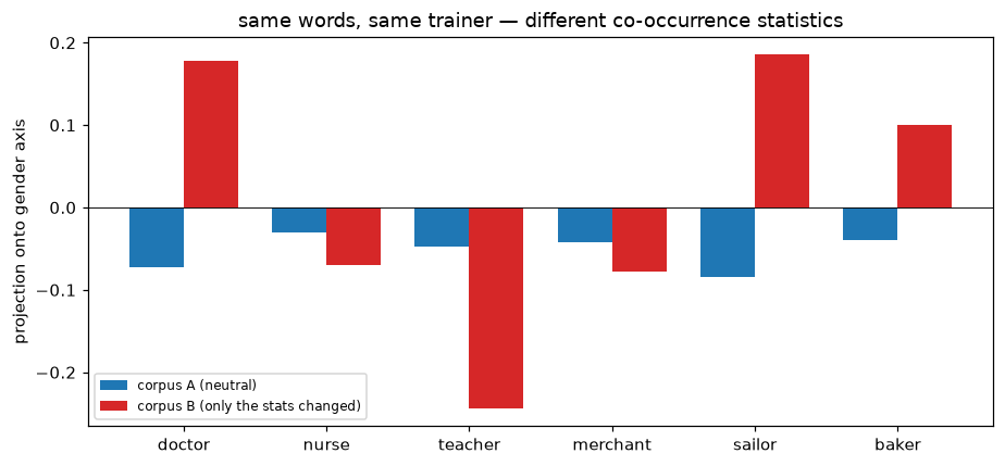
In our default corpus, professions co-occur with male and female pronouns at exactly 50/50. Now regenerate the world with one statistic flipped: doctor keeps masculine company (90% he/his) and sailor 85%, while nurse gets feminine company (95% she/her) and teacher 90% — everything else unchanged (merchant, baker stay neutral as controls). Same code, same words, different counts. Then retrain and measure each profession’s projection onto the gender axis (the mean of the eight male−female unit differences, the same axis the PCA arrows showed) — before and after.
If the vectors move, an embedding is not a thought about women and men; it is the corpus’s co-occurrence statistics wearing a trench coat. This is why Bolukbasi et al.’s 2016 findings on real word2vec (man : computer programmer :: woman : homemaker) surprised exactly nobody who had read Levy–Goldberg carefully: the model can only be a mirror. (Their proposed fix — geometric debiasing — also only makes sense once you see the bias as a direction in this space. Which we now have, concretely.)
def gender_dir(E):
    E0 = normed(E)
    d = np.mean([E0[w2i[m]] - E0[w2i[f]] for m, f in GENDER_PAIRS], axis=0)
    return d / np.linalg.norm(d)

sents_B = generate_corpus(12000, seed=0, profession_bias={"doctor": 0.90, "nurse": 0.05, "sailor": 0.85, "teacher": 0.10})
w2i_B, vocab_B, freq_B = build_vocab(sents_B)
assert vocab_B == vocab
pairs_B = []
for s in [[w2i_B[w] for w in sent] for sent in sents_B]:
    for i, c in enumerate(s):
        for j in range(max(0, i - WINDOW), min(len(s), i + WINDOW + 1)):
            if i != j:
                pairs_B.append((c, s[j]))
pairs_B = np.array(pairs_B)
E_B, U_B = train_sgns(pairs_B, freq_B, D, epochs=10, lr=0.05, seed=1, verbose=False)

gA = gender_dir(E); gB = gender_dir(E_B)
proj = [(pr, float(normed(E)[w2i[pr]] @ gA), float(normed(E_B)[w2i[pr]] @ gB)) for pr in PROF]
print(f"{'profession':<12} {'proj on gender axis, corpus A (neutral)':>24} {'corpus B (skewed)':>20}")
for pr, a, b in proj:
    print(f"{pr:<12} {a:>+24.3f} {b:>+20.3f}")

fig, ax = plt.subplots(figsize=(8.5, 4))
xpos = np.arange(len(PROF))
ax.bar(xpos - 0.19, [p[1] for p in proj], width=.38, label="corpus A (neutral)", color="tab:blue")
ax.bar(xpos + 0.19, [p[2] for p in proj], width=.38, label="corpus B (only the stats changed)", color="tab:red")
ax.axhline(0, color="k", lw=.6)
ax.set_xticks(xpos, PROF); ax.set_ylabel("projection onto gender axis")
ax.set_title("same words, same trainer — different co-occurrence statistics")
ax.legend(fontsize=8)
fig.tight_layout(); fig.savefig(FIGS / "bias_mirror.png", dpi=140, bbox_inches="tight"); plt.show()
save_ckpt(CKPT, "bias_mirror", metrics={}, E_A=E, E_B=E_B)
profession   proj on gender axis, corpus A (neutral)    corpus B (skewed)
doctor                         -0.073               +0.178
nurse                          -0.031               -0.070
teacher                        -0.047               -0.244
merchant                       -0.042               -0.078
sailor                         -0.084               +0.185
baker                          -0.040               +0.100
PosixPath('checkpoints/lab21/bias_mirror.npz')
9. What we established, and where the cracks are
Meaning is compressible co-occurrence. SGNS needed no semantics: §5 measured it tracking the closed-form PMI matrix (and one SVD reproduced its neighbors without a single gradient step). The geometry that “knows” king from queen is a lossy, denoising projection of count ratios — powerful precisely because it generalizes the raw matrix instead of memorizing it.
The cracks to notice before the next lab.
- Static: one vector per word, so sense-merging is structural — covered in your own Word2Vec static-limitation notebook (polysemy, antonyms). The fix isn’t a bigger table; it’s context-dependent vectors — attention, later in this series.
- Window-blind:
king rulesandrules kinggive the same pairs. Word order is thrown away at the input — RNNs (next lab) put it back, at a price. - UNK: every unseen word is a shrug. Subword tokenization (BPE/SentencePiece) fixes it and changes the interface between text and network — we’ll pick it up before the transformer lab.
Reading:
- Mikolov et al., Efficient Estimation of Word Representations in Vector Space (2013) — the origin.
- Levy & Goldberg, Neural Word Embedding as Implicit Matrix Factorization (NeurIPS 2014) — §5’s proof; the single most clarifying paper about word2vec ever written.
- Pennington et al., GloVe (2014) — what happens when you factorize the count matrix on purpose: one objective, no sampling.
- Bolukbasi et al., Man is to Computer Programmer as Woman is to Homemaker? (2016) — §8 with real data, plus a geometric debiasing method.
- Firth, “A synopsis of linguistic theory” (1957) — the eight words that started it all.
Next (Lab 2.2): a language model without attention — char-level RNN in NumPy, backprop through time written by hand, and the measured version of “vanishing gradients”: a synthetic memory task where we watch the gradient signal die as the dependency grows, step by step, before any LSTM shows up to save it.
Reproduce
cd labs/ml/lm-internals
# reuses the mnist-internals venv (same pinned deps); kernel "Python (lm-labs shared)"
jupyter lab    # open 01_how_word_vectors_learn_to_mean.ipynb
Artifacts: checkpoints/lab21/ (sgns_main.npz — E/U/PMI/counts, dim_sweep.npz, bias_mirror.npz + manifest.json), figures/lab21/*.png.
print("checkpoints written this lab:")
for e in manifest(CKPT):
    print(f"  {e['name']:<12} metrics={e['metrics']}")
checkpoints written this lab:
  sgns_main    metrics={'dim': 16, 'pearson_vs_pmi': 0.952}
  dim_sweep    metrics={'2': {'analogy_exact': 0.06, 'gender_acc': 0.12, 'pearson': 0.618}, '4': {'analogy_exact': 0.0, 'gender_acc': 0.12, 'pearson': 0.775}, '8': {'analogy_exact': 0.12, 'gender_acc': 0.56, 'pearson': 0.911}, '16': {'analogy_exact': 0.12, 'gender_acc': 1.0, 'pearson': 0.94}, '32': {'analogy_exact': 0.12, 'gender_acc': 1.0, 'pearson': 0.948}, '64': {'analogy_exact': 0.12, 'gender_acc': 1.0, 'pearson': 0.956}}
  bias_mirror  metrics={}